Zyklusbezogener β-Servicegrad
1 −
E
(
t
X
j=τ
F
j
(q
τ t
)
)
E
(
t
X
j=τ
D
j
)
≥ β
⋆
c
τ = 1, 2, . . .
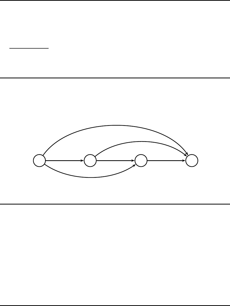
Netzwerk
1 2 3 4
E{C
12
} E{C
23
(P
2
)} E{C
34
(P
3
)}
E{C
24
(P
2
)}
E{C
14
}
E{C
13
}
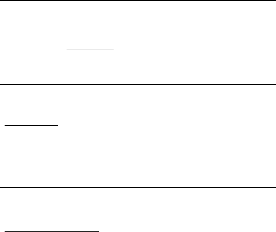
Erwarteter Lagerbestand
am Ende der Periode t
Q
(t)
– cumulated production quantity in periods 1 to t
Y
(t)
– cumulated demand in periods 1 to t
E{I
p
t
} =
Z
Q
(t)
0
(Q
(t)
− y) · f
Y
(t)
(y) · dy
=Q
(t)
− E{Y
(t)
} + G
1
Y
(t)
(Q
(t)
)
117
Kantengewicht
E{C
τ t
} = s + h ·
t−1
X
ℓ=τ
E
"
I
p
τ −1
(P
τ
) + q
opt
τ t
−
ℓ
X
i=τ
D
i
#
+
• q
opt
τ t
ist die minimale Los gr¨oße, die ben¨otigt wird, um β
c
in Periode t zu erreichen
• q
opt
τ t
h¨angt vom Anfangsbestand in Periode τ ab
• q
opt
τ t
kann mit einem einfachen Suchverfahren bestimmt werden
• Wichtig: Der physischen Bestand E
I
p
τ −1
(P
τ
)
am Anfang der Periode τ h¨angt von den ku-
mulierten Produktionsmengen bis zur Periode τ − 1 ab
Optimale Losgr¨oße
q
opt
τ t
(β
c
) = min
q
τ t
1 −
E
(
t−1
X
i=τ
B
i
(q
τ t
)
)
E
(
t−1
X
i=τ
D
i
)
≥ β
c
Optimale Losgr¨oße
Daten
t E{D
t
} σ
D
t
1 200 60
2 50 15
3 100 30
4 300 90
5 150 45
6 200 60
Optimale Losgr¨oße
Suchverfahren
q
1
Q
(1)
G
1
Y
(1)
β
c
230 230 11.87 0.9407
231.87 231.87 11.30 0.9435
233.17 233.17 10.92 0.9454
.
.
.
.
.
.
.
.
.
236.44 236.44 10.00 0.9500
118

28.3 Dynamische Losgr¨oßenheuristik
General heuristic procedure
1: τ := 1
2: while (τ < T ) do
3: t := τ
4: while (t < T ) do
5: if (C
τ t
≤ C
τ,t+1
) then
6: t := t + 1
7: else
8: Make current lotsize for period τ permanent.
9: τ := t + 1
10: end if
11: end while
12: end while
Modifiziertes Silver-Meal-Verfahren
Kriterium
E{C
τ t
} =
s + h ·
t
X
ℓ=τ
E
"
I
τ −1
(P
τ −1
) + q
∗
τ t
−
ℓ
X
i=τ
D
i
#
+
t − τ + 1
P
τ −1
ist der Produktionsplan von Periode 1 bis zur Periode (τ − 1) und τ ist die letzte Produktionspe-
rioden vor Periode t.
Modifiziertes Silver-Meal-Verfahren
Fehlmenge
E{I
f,Prod
t
} = E{
h
Y
(t−1)
− Q
(t)
i
+
} = G
1
Y
(t−1)
(Q
(t)
)
E{I
f,End
t
} = E{
h
Y
(t)
− Q
(t)
i
+
} = G
1
Y
(t)
(Q
(t)
)
E{B
t
} = E{I
f,End
t
} − E{I
f,Prod
t
}
Modifiziertes Silver-Meal-Verfahren: Kostenberechnung
Lagerbestand
E{I
p
t
} = E{
h
Q
(t)
− Y
(t)
i
+
}
E{I
p
t
} = Q
(t)
− E{Y
(t)
+ E{I
f,End
t
}
119

Modifiziertes Silver-Meal-Verfahren
Beispiel
t E{D
t
} σ
D
t
1 20 6
2 80 24
3 160 48
4 85 25.5
5 120 36
6 100 30
β = 0.99 ; s = 500; h = 1
Modifiziertes Silver-Meal-Verfahren
Beispiel
τ t E{D
t
} C
τ t
q
t
Erwartete Kosten pro Z yklus
1 1 20 508.86 28.66
2 80 324.02 133.52 648.04
3 160 369.61
3 3 160 582.32 207.20
4 85 374.24 291.99
5 120 362.20 417.47 1086.61
6 100 370.21
6 6 100 639.86 152.87 639.86
Modifiziertes Silver-Meal-Verfahren
Rechenschritte
τ = 1, t = 1 :
E{Y
(1)
} = 20; σ{Y
(1)
} = 6
Q
(1)
(β
c
= 0.99) = 28.66 kumulierte Produktionsmenge
q
opt
11
= 28.66 Losgr¨oße
E{I
f,Prod
1
} = 0 Fehlbestand am Anfang der Periode 1
E{I
f,End
1
} = Φ
1
(v =
28.66−20
6
) · 6
= 0.0334 · 6 = 0.20 Fehlbestand am Ende der Periode 1
E{I
p
1
} = 28.66 − 20 + 0.20 = 8.86 physischer Lagerbestand am Ende der Perio de 1
C
11
=
500+8.86
1
= 508.86 erwartete Kosten pro Perio de f¨ur t = 1
120
Modifiziertes Silver-Meal-Verfahren
Rechenschritte
τ = 1, t = 2 :
E{Y
(2)
} = 100; σ{Y
(2)
} = 24.74
Q
(2)
(β
c
= 0.99) = 133.52 kumulierte Produktionsmenge
q
opt
12
= 133.52 Losgr¨oße
E{I
f,Prod
1
} = 0 Fehlbestand am Anfang der Periode 1
E{I
f,End
1
} = Φ
1
(v =
133.52−20
6
) · 6 = 0 Fehlbestand am Ende der Periode 1
E{I
p
1
} = 133.52 − 20 + 0.0 = 113.52 physischer Lagerbestand am Ende der Perio de 1
E{I
f,End
2
} = Φ
1
(v =
133.52−100
24.74
) · 24.74
= 0.0405 · 24.74 = 1.0 Fehlbestand am Ende der Periode 2
E{I
p
2
} = 133.52 − 100 + 1.0 = 34.52 physischer Lagerbestand am Ende der Perio de 2
C
12
=
500+(113.52+34.52)
2
= 324.02 erwartete Kosten pro Perio de f¨ur t = 2
Modifiziertes Silver-Meal-Verfahren
Rechenschritte
τ = 3, t = 3 :
E{Y
(3)
} = 260; σ{Y
(3)
} = 54
Q
(3)
(β
c
= 0.99) = 340.72 kumulierte Produktionsmenge
q
opt
33
= 340.72 − 133.52 = 207.20
E{I
f,Prod
3
} = Φ
1
(v =
340.72−100
24.74
) · 24.74 = 0 Fehlbestand am Anfang der Periode 3
121