
Teil IV
Losgr¨oßen- und Materialbedarfsplanung I
10 Programmorientierte Materialbedarfsrechnung
Daten
• Hauptproduktionsprogramm
• Erzeugnisz usammenhang
• Durchlaufzeit
• Lagerbest¨ande
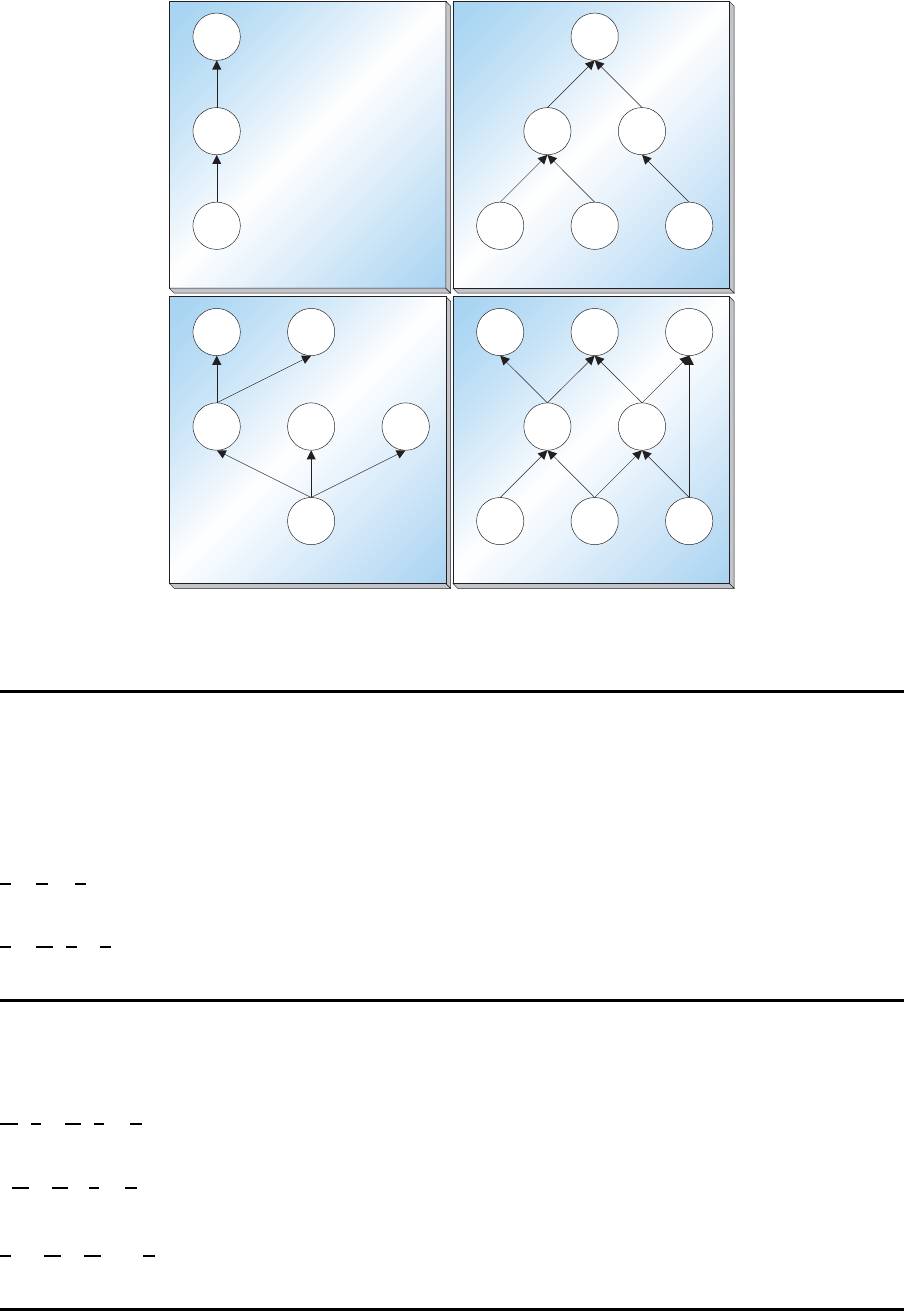
10.1 Darstellung des Erzeugniszusammenhangs
Typen von Erzeugnisstrukturen
• lineare Erzeugnisstruktur
• konvergierende Erzeugnisstruktur
• divergierende Erzeugnisstruktur
• generelle Erzeugnisstruktur
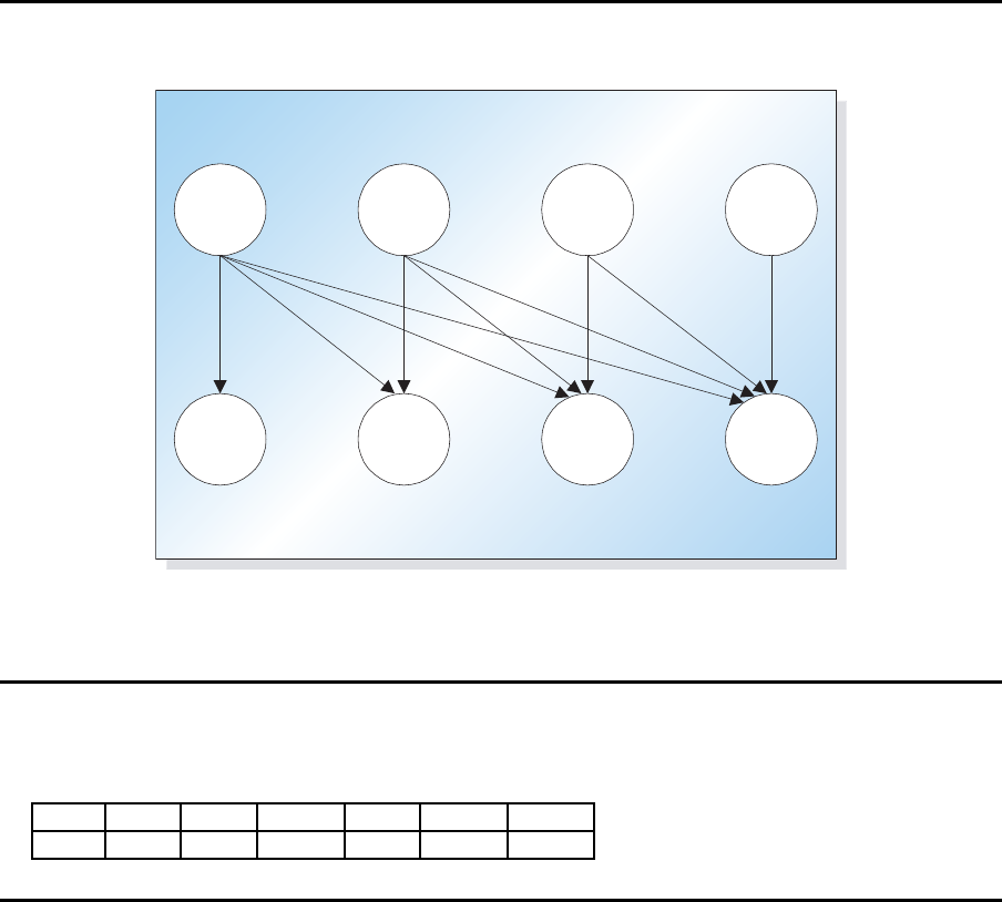
Gozintographen f¨ur unterschiedliche Erzeugnisstrukturen
28
P1
B1
E1
P1 P2
P3 P4B1
E1
P1 P2 P3
B1 B2
E1 E2 E3
P1
B1 B2
E1 E2 E3
b) konvergierenda) linear
c) divergierend d) generell
10.2 L¨osung eines linearen Gleichungssystems
Lineares Gleichungssystem I
r
k
= y
k
+ d
k
k = 1, 2, ..., K
r = y + d
r = A · r + d
Lineares Gleichungssystem II
E · r −A · r = d
(E − A) · r = d
r = (E − A)
−1
· d
29
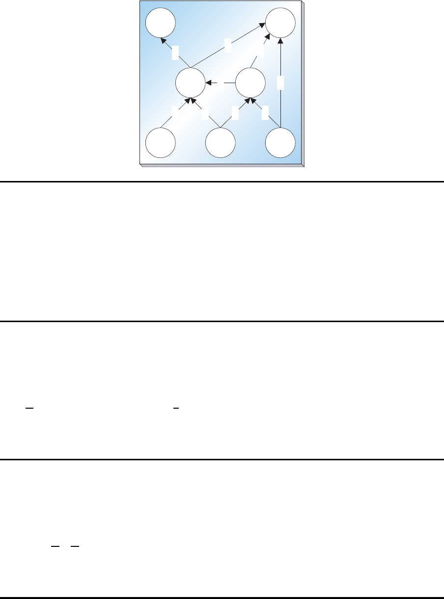
Gozintograph
P1
E1
B1 B2
E3
2
P2
E2
3
1
2
1
4
536
Lineares Gleichungssystem III
r
E1
= 0 · r
E1
+ 0 · r
E2
+ 0 · r
E3
+ 6 · r
B1
+ 0 · r
B2
+ 0 · r
P 1
+ 0 · r
P 2
+ 0
r
E2
= 0 · r
E1
+ 0 · r
E2
+ 0 · r
E3
+ 3 · r
B1
+ 5 · r
B2
+ 0 · r
P 1
+ 0 · r
P 2
+ 0
r
E3
= 0 · r
E1
+ 0 · r
E2
+ 0 · r
E3
+ 0 · r
B1
+ 1 · r
B2
+ 0 · r
P 1
+ 4 · r
P 2
+ 0
r
B1
= 0 · r
E1
+ 0 · r
E2
+ 0 · r
E3
+ 0 · r
B1
+ 0 · r
B2
+ 2 · r
P 1
+ 3 · r
P 2
+ 20
r
B2
= 0 · r
E1
+ 0 · r
E2
+ 0 · r
E3
+ 2 · r
B1
+ 0 · r
B2
+ 0 · r
P 1
+ 1 · r
P 2
+ 40
r
P 1
= 0 · r
E1
+ 0 · r
E2
+ 0 · r
E3
+ 0 · r
B1
+ 0 · r
B2
+ 0 · r
P 1
+ 0 · r
P 2
+ 100
r
P 2
= 0 · r
E1
+ 0 · r
E2
+ 0 · r
E3
+ 0 · r
B1
+ 0 · r
B2
+ 0 · r
P 1
+ 0 · r
P 2
+ 80
Lineares Gleichungssystem IV
A =
0 0 0 6 0 0 0
0 0 0 3 5 0 0
0 0 0 0 1 0 4
0 0 0 0 0 2 3
0 0 0 2 0 0 1
0 0 0 0 0 0 0
0 0 0 0 0 0 0
d =
0
0
0
20
40
100
80
E1
E2
E3
B1
B2
P 1
P 2
Technologiematrix
(E − A) =
1 0 0 −6 0 0 0
0 1 0 −3 −5 0 0
0 0 1 0 −1 0 −4
0 0 0 1 0 −2 −3
0 0 0 −2 1 0 −1
0 0 0 0 0 1 0
0 0 0 0 0 0 1
30
Verflechtungsbed arfsmatrix
(E − A)
−1
=
1 0 0 6 0 12 18
0 1 0 13 5 26 44
0 0 1 2 1 4 11
0 0 0 1 0 2 3
0 0 0 2 1 4 7
0 0 0 0 0 1 0
0 0 0 0 0 0 1
Verflechtungsbed arf E2 → P2
v
E2,P 2
= a
E2,B1
· a
B1,P 2
+ a
E2,B2
· a
B2,B1
· a
B1,P 2
+ a
E2,B2
· a
B2,P 2
= 3 · 3 + 5 · 2 · 3 + 5 · 1 = 44
Gozintograph
P1
E1
B1 B2
E3
2
P2
E2
3
1
2
1
4
5
36
P1
E1
B1 B2
E3
2
P2
E2
3
1
2
1
4
536
P1
E1
B1 B2
E3
2
P2
E2
3
1
2
1
4
536
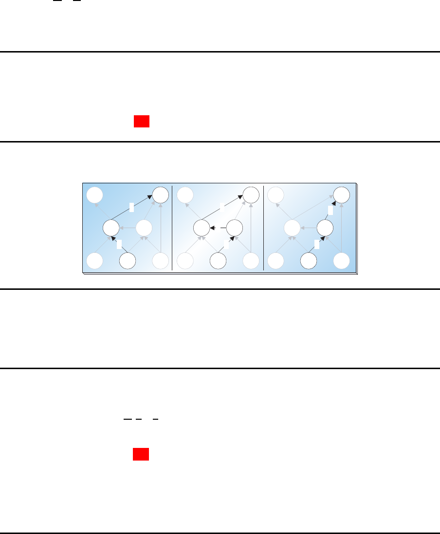
Verflechtungsbed arf
w
ij
=
s−1
Q
m=1
a
i
m
,i
m+1
∀ij
Gesamtbedarf
V ·d = r
1 0 0 6 0 12 18
0 1 0 13 5 26 44
0 0 1 2 1 4 11
0 0 0 1 0 2 3
0 0 0 2 1 4 7
0 0 0 0 0 1 0
0 0 0 0 0 0 1
·
0
0
0
20
40
100
80
=
2760
6580
1360
460
1040
100
80
E1
E2
E3
B1
B2
P 1
P 2
31
Lagerbilanzgleichung
y
k,t−1
+ q
k,t−z
k
−
X
i∈N
k
a
ki
· q
it
− y
kt
= d
kt
k = 1, 2, ..., K; t = 1, 2, ..., T
32
11 Das dynamische Einprodukt-Losgr¨oßenproblem
11.1 Modellformulierungen
Modell SLULSP
Wagner-Whitin-Problem
Minimiere Z =
T
X
t=1
s · γ
t
+ h · y
t
+ p
t
·q
t
u. B. d. R.
y
t−1
+ q
t
− y
t
= d
t
t = 1, 2, ..., T
q
t
− M · γ
t
≤ 0 t = 1, 2, ..., T
D
ti
=
i
X
j=t
d
j
t, i = 1, 2, ..., T ; i ≥ t
q
t
− D
tT
· γ
t
≤ 0 t = 1, 2, ..., T
Es gilt die Optimalit¨atsbedingung:
q
t
·y
t−1
= 0 t = 1, 2, ..., T
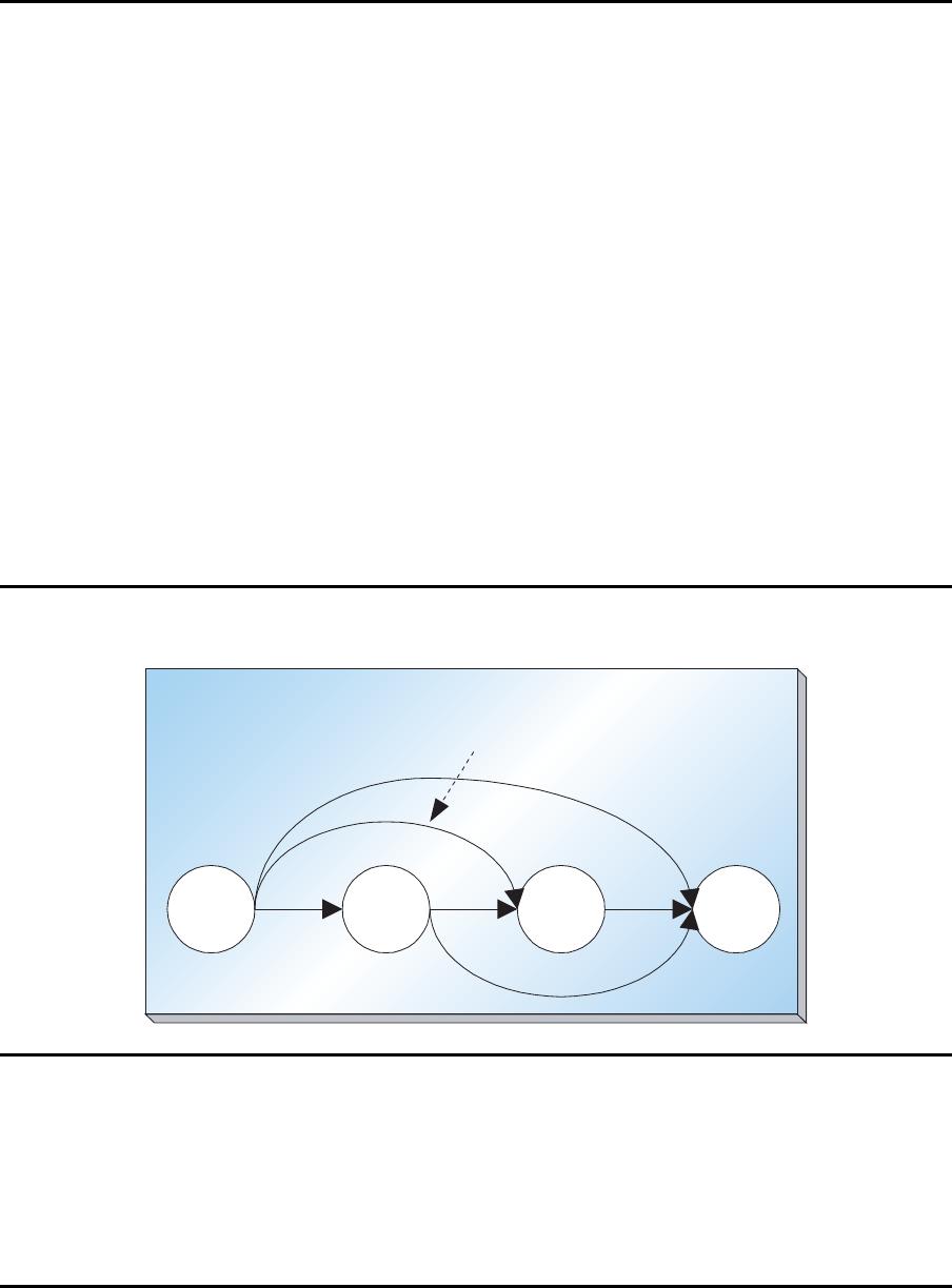
Netzwerkdarstellung des dynamischen Losgr¨oßenproblems
0 1 2 3
Bereitstellung des Bedarfs der Perioden
1 und 2 zu Beginn der Periode 1
Kosten eines Pfeils
R¨ustkosten + gesamte Lagerkosten
w
τ t
= s + h ·
t
X
j=τ +1
(j − τ − 1) · d
j
33
Standortformuli erung
Modell SPLP
Minimiere Z =
T
X
τ =1
s · γ
τ
+
T
X
τ =1
T
X
t=τ
h
τ t
·δ
τ t
u. B. d. R.
t
X
τ =1
δ
τ t
= 1 t = 1, 2, . . . , T
δ
τ t
≤ γ
τ
τ = 1, 2, . . . , T ; t = τ, τ + 1, . . . , T
δ
τ t
, γ
τ
∈ {0, 1} τ = 1, 2, . . . , T ; t = τ, τ + 1, . . . , T
h
τ t
= h · d
t
·(t − τ) τ = 1, 2, . . . , T ; t = τ, τ + 1, . . . , T
Standortformuli erung
Modell SPLP
1 2 3 4
Produktionsperioden ("potentielle Standorte")
1 2 3 4
Bedarfsperioden ("Nachfrageorte")
11.2 Exakte L¨osung mit dynamischer Optimierung
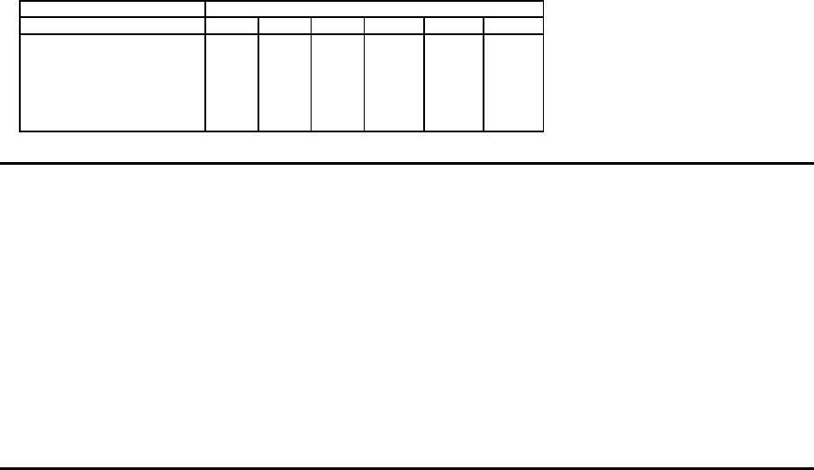
Beispiel
Bedarfsmengen
t 1 2 3 4 5 6
d
t
20 80 160 85 120 100
34
Kosten
c
τ j
= s + h ·
j
X
t=τ +1
(t − τ ) · d
t
τ ≤ j
letzte Verbrauchsperiode (j)
Bereitstellungsperiode (τ) 1 2 3 4 5 6
1 500 580 900 1155 1635 2135
2 – 500 660 830 1190 1590
3 – – 500 585 825 1125
4 – – – 500 620 820
5 – – – – 500 600
6 – – – – – 500
Dynamische Programmierung
C
6
= C
i
+ c
i+1,6
i = 1, 2, ..., 5
z. B.
C
6
= C
5
+ c
66
f
i
= min
1≤l≤i
{f
l−1
+ c
li
} i = 1, 2, ...T
P
6
= ( P
5
, p
66
)
P
6
= ( P
4
, p
56
)
P
6
= ( P
3
, p
46
)
P
6
= ( P
2
, p
36
)
P
6
= ( P
1
, p
26
)
P
6
= ( p
16
)
35

Aktueller Planungshorizont j = 1
f(0)+c(1,1) = 0+ 500 = 500
Minimale Ko sten f¨ur j = 1 f(1) =500
Optimale Losgr¨oßen:
q( 1): 20
Aktueller Planungshorizont j = 2
f(0)+c(1,2) =0+580 =580
f(1)+c(2,2) = 500+ 500 = 1000
Minimale Ko sten f¨ur j = 2 f(2) =580
Optimale Losgr¨oßen:
q( 1): 100
Aktueller Planungshorizont j = 3
f(0)+c(1,3) =0+900 =900
f(1)+c(2,3) =500+660 =1160
f(2)+c(3,3) = 580+ 500 = 1080
Minimale Ko sten f¨ur j = 3 f(3) =900
Optimale Losgr¨oßen:
q( 1): 260
Aktueller Planungshorizont j = 4
f(0)+c(1,4) =0+1155 =1155
f(1)+c(2,4) =500+830 =1330
f(2)+c(3,4) =580+585 =1165
f(3)+c(4,4) = 900+ 500 = 1400
Minimale Ko sten f¨ur j = 4 f(4) =1155
Optimale Losgr¨oßen:
q( 1): 345
Aktueller Planungshorizont j = 5
f(0)+c(1,5) =0+1635 =1635
f(1)+c(2,5) =500+1190 =1690
f(2)+c(3,5) =580+825 =1405
f(3)+c(4,5) =900+620 =1520
f(4)+c(5,5) = 1155+ 500 = 1655
Minimale Ko sten f¨ur j = 5 f(5) =1405
Optimale Losgr¨oßen:
q( 1): 100
q( 3): 365
Aktueller Planungshorizont j = 6
f(0)+c(1,6) =0+2135 =2135
f(1)+c(2,6) =500+1590 =2090
f(2)+c(3,6) =580+1125 =1705
f(3)+c(4,6) =900+820 =1720
f(4)+c(5,6) =1155+600 =1755
f(5)+c(6,6) = 1405+ 500 = 1905
Minimale Ko sten f¨ur j = 6 f(6) =1705
Optimale Losgr¨oßen:
q( 1): 100
q( 3): 465
11.3 Heuristische L¨osungsverfahren
Heuristische L¨osungsverfahren
Siehe Vorlesung Produktio n und Logistik.
36
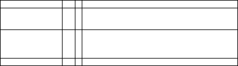
t d
t
j c
per
τ j
1 20 1 500.000
1 80 2 290.000
Losgr¨oß e in Periode 1: 100
3 160 3 500.00
3 85 4 292.500
3 120 5 275.000
Losgr¨oß e in Periode 3: 365
6 100 6 500.00
37